My larger goal is explaining the circuits by which a transformer trained for natural language processing parses ambiguous language– in particular, homonyms. First, it is important to think about what it might mean to parse a word whose definition is ambiguous. Two words with the same spelling are necessarily similar in their input representation. If they are to be processed as having one of two distinct meanings (for example, based on their surrounding context), then across the layers of the network, this one cluster of words might come to be represented as two separate clusters. If this model were correct, representations of two instances of a homonym should share a cluster in a later layer of the network if and only if they share the same underlying definition. But what should it mean to share a cluster? In the following post, I explain two related metrics by which we can evaluate how differently two sets of points are represented. To establish an intuition, we first look to a more visual example: parsing images based on what objects are in them.

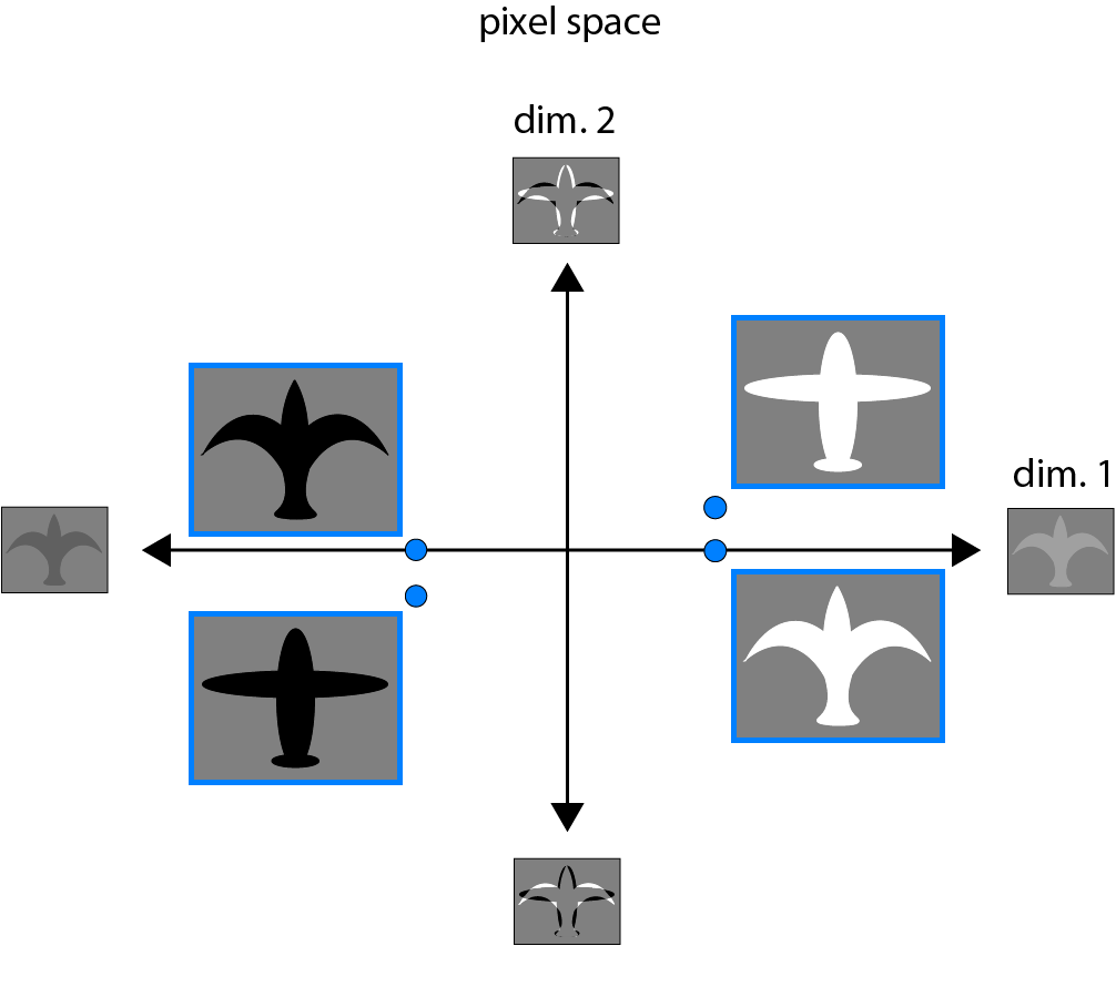
The goal of a deep learning model can be thought of as learning an arbitrary transformation between inputs and outputs. We will define “semantically distinct” inputs as inputs for which a well-trained model should respond with different outputs, and “semantically similar” inputs as inputs for which a well-trained model should respond with the same or similar outputs. In many problems in AI, classes of semantically distinct inputs may be “tangled,” in the sense that two inputs that should evoke the same response are superficially different, by some reasonable metric, while two inputs that should evoke different responses are superficially similar. As an example, in a network for discriminating birds from planes, an image of a white vs. a black bird may be far apart in pixel space, but both should be labeled “bird.” If we consider in addition an image of a white vs. a black plane, each one’s nearest neighbor in pixel space may be the white and black bird, respectively, but these nearest neighbor pairs should be assigned distinct labels. In the example below, in pixel space, the categories of “bird” and “plane” are linearly inseparable.

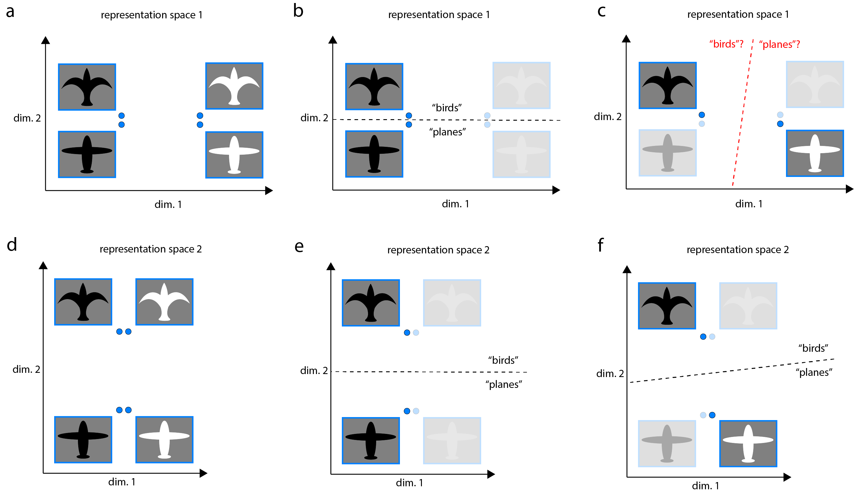
To distinguish these semantically distinct input classes, a model must “untangle” these tangled input representations, learning representations in which they are linearly separable. However, not all linearly separable representations are created equal. If a representation is suboptimal, training a linear classifier that is able to generalize well might require a large amount of data. In “representation space 1” below, “birds” and “planes” are linearly separable, but objects are represented nearby distinct objects of the same color (a). A linear classifier trained on the representation of just one bird and one plane might generalize well (b) or poorly (c) based on whether it lucked into a good pair of training examples (e.g. the black bird and black plane in (b), as opposed to the black bird and white plane in (c)). Because color in this case is not a useful feature for the task of discriminating birds from planes, this representation would seem suboptimal in that it represents color so strongly.

On the other hand, in “representation space 2” below, “birds” and “planes” are linearly separable, and objects are represented nearby semantically similar objects, regardless of color (d). Distinctions related to the “nuisance” feature of color are almost entirely projected out. A linear classifier trained on any bird-plane pair is likely to generalize well to the others (e,f). It would seem to me that separability between semantically distinct inputs that is learnable in the data-limited context may be important for efficiently training new tasks during fine-tuning, or for succeeding at few-shot learning tasks.

In practice, linear separability in the non-data-limited context can be quantified, familiarly, by training a logistic regression model on one half of a full dataset, and testing performance on the other half. To quantify linear separability in the data-limited context, we first consider a random example from each input class. The success probability of a linear classifier trained on these two data points can be calculated as the probability that the representation of a third random example, of either input class, is closer to the representation of the input sharing its class. The average success probability of such a linear classifier over all possible such triplets of distinct inputs turns out to have a simple mathematical form. We start with the distance matrix \(D\), where each entry \(D_{ij}\) is the distance in representation space between the \(i\)th and \(j\)th input. For each row \(i\), we compute the AUROC between distances to distinct points in the same semantic class, and points in the opposite semantic class, and then average across rows. A derivation is below, for those interested.

With the tools now in hand for thinking about what it would mean for semantically distinct input representations to be “untangled,” we can now think about what sets of representations a deep learning model might want to untangle. In the context of computer vision, we can imagine the set of semantically similar inputs to take the form of a continuous manifold. For the purpose of a particular image identification or captioning task, there are continuous deformations in lighting, position, scale, and 3D pose of an object, among other attributes, that a well-trained model might effectively ignore. In fact, representations in successive layers of deep CNNs are increasingly invariant to these types of continuous transformations, in the sense of object representations being linearly separable despite them. Circuit mechanisms for such invariance are beginning to be understood. Similarly with representations in a higher primate visual area, area IT of the ventral stream.

In the context of natural language processing, what types of semantically distinct input might a deep learning model want to untangle? Homonyms are a good example of inputs that have a similar representation to start (in the sense of identical spelling), but that we intuitively feel should be separable into distinct classes. As a first example, we will take two homonyms– “pack” as a verb, and “pack” as a noun. To do many language tasks well, the fact that these two words are spelled the same is of little importance: mostly, they should be represented as different words with different meanings, in much the same way as if they had totally unrelated spellings. We can think of them as the flip-side of the two different images, distant in pixel space, both similarly labeled as “bird”: homonyms are two very similar sets of inputs, that should be mapped to quite different outputs. More to come in the next post.

Derivation

Given the representation of a fixed third point \(x_3\), we can compute its distance to the representation of each other point \(x_1\) in its class, \(d(x_1,x_3)\). We will define the data distribution of such distances as \(p(\Delta_1 | x_3)=P\left(d(x_1,x_3)=\Delta_1 \right)\), where \(P\) denotes probability. Similarly, for the representations of points in the opposite class, we define the data distribution of distances to be \(q(\Delta_2 | x_3)=P\left(d(x_2,x_3)=\Delta_2 \right)\). \(P(success)\) of the linear classifier is equivalent to \(P(\Delta_1<\Delta_2)\), where \(\Delta_1 \sim p\), \(\Delta_2 \sim q\): \[ \label{label} P(success | x_3) = \int_{-\infty}^{\infty} q(\Delta_2 | x_3) \int_{-\infty}^{\Delta_2} p(\Delta_1 | x_3) d\Delta_1 d\Delta_2. \] Meanwhile, to compute the AUROC between \(p\) and \(q\), we define \[ X(\Delta) = \int_{-\infty}^{\Delta} q(\Delta’ | x_3) d\Delta’, \] \[ Y(\Delta) = \int_{-\infty}^{\Delta} p(\Delta’ | x_3) d\Delta’, \] such that \[ AUROC(p,q|x_3) = \int_0^1 Y dX. \] Now, using \(dX = q(\Delta|x_3) d\Delta\), we have \[ AUROC(p,q|x_3) = \int_{-\infty}^{\infty} q(\Delta_2 |x_3) \int_{-\infty}^{\Delta_2} p(\Delta_1 | x_3) d\Delta_1 d\Delta_2, \] identical to the above. One can then compute \(P(success)\) by averaging over all points \(x_3\) in the dataset, equivalent to integrating \[P(success) = \int AUROC(p,q|x_3) P(x_3) dx_3. \]